|
Here we explain a simple way to use of gnuplot for a technical
paper submission. There are many formats and methods to submit
your paper, and those usually depend on a society rule. So that
the technique here is an example.
A common way to send your graphs to an editorial office is
probably to prepare your graphs on separate sheets and attach
captions of figures. We generate them with LaTeX.
- General notes to make figures
- TeX
- Change the direction of figure
- Make a separate Postscript page
- done
Firstly all your figures are prepared by gnuplot in the EPS format.
- Your graphs are generated by the set term postscript eps
enhanced commands. If they accept a color figure, add the
color option.
- Use large fonts for tics, label, and
legend.
When your thesis is printed in a journal, the size of your figures
are usually reduced to fit the page. So that you should avoid to
use small fonts because they become very small and hard to read.
The best size may be depend on the figure size and journal page width.
- When you want to include several figures in one drawing,
make them in the same size.
- You can also combine some figures generated by another software
if those are in the EPS format.
Here we prepared some files those were made with gnuplot.
Each figure is drawn on a separate sheet --- one A4-size paper
contains one figure. The figure number, caption, and the author's name
are shown in a margin on each sheet.
From the four EPS files above, we make a A4-size Postscript file
which contains figure pages. This can be done with the LaTeX2e
graphics (graphicx) package. Let's make a TeX file "figure.tex", and
import EPS files in it. The next shows the top part of this file.
\documentclass[12pt]{article}
\oddsidemargin   0mm
\evensidemargin  0mm
\topmargin       0mm
\headheight      0mm
\headsep         0mm
\topskip         0mm
\textwidth     160mm   % 210 - 25x2 mm
\textheight    235mm   % 297 - 30x2 -2 mm
\baselineskip  12pt    % single space
\usepackage[dvips]{graphics}
\begin{document}
\pagestyle{empty}
The EPS files are imported by the \includegraphics
command, and adjust (enlarge) the figure width by \resizebox
. At the top of each page, the figure number, author's name and
affiliation are written. In the next example those infomation is
top/right aligned.
\begin{flushright}
Fig.~1~:~ Kawano, T. (LANL)
\end{flushright}
\vskip 1cm
\begin{center}
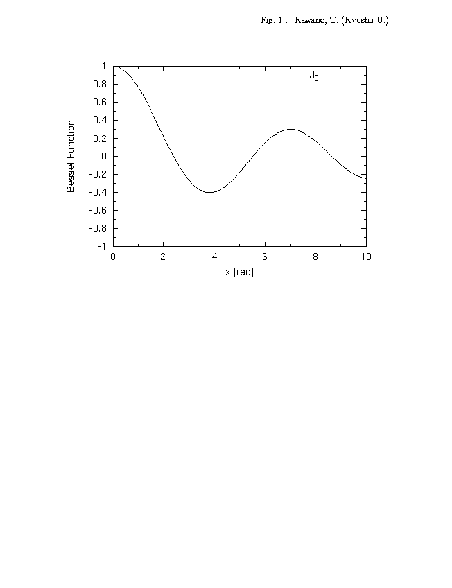
\resizebox{150mm}{!}{\includegraphics{besj0.eps}}
\end{center}
\clearpage
If you want to include the figure caption, use figure
environment. In this case you can use a figure label, so the second
line (figure number) can be generated automatically.
\begin{flushright}
  Fig.~\ref{besj0}~:~ Kawano, T. (LANL)
\end{flushright}
\vskip 1cm
\begin{figure}[b!]
  \begin{center}
    \resizebox{150mm}{!}{\includegraphics{besj0.eps}}
    \caption{Bessel function, $J_0$.}
    \label{besj0}
  \end{center}
\end{figure}
\clearpage
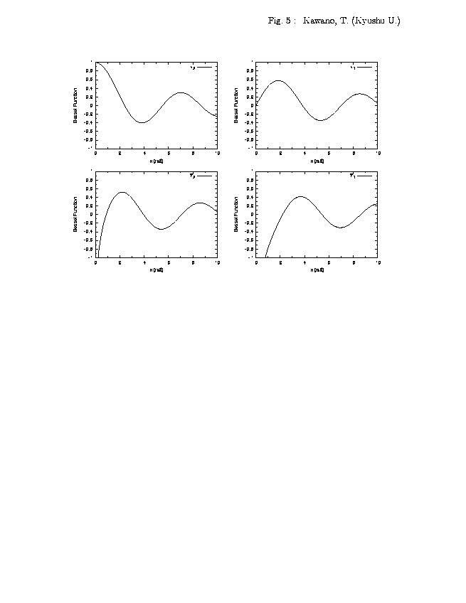
To include several plots in one figure, align those plots by the
tabular environment. To combine the four EPS in one
figure:
\begin{flushright}
  Fig.~5~:~ Kawano, T. (LANL)
\end{flushright}
\vskip 1cm
\begin{center}
  \begin{tabular}{cc}
     \resizebox{70mm}{!}{\includegraphics{besj0.eps}} >
     \resizebox{70mm}{!}{\includegraphics{besj1.eps}} \\
     \resizebox{70mm}{!}{\includegraphics{besy0.eps}} >
     \resizebox{70mm}{!}{\includegraphics{besy1.eps}} \\
  \end{tabular}
\end{center}
\clearpage
Cares must be made for the size of letters, because the letter
size becomes very small in this case.
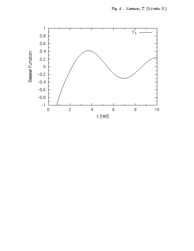
In order to change the direction of figure, rotate
EPS by \rotatebox . Your figure becomes wider.
In the following example the width of figure (printed length)
was enlarged to 20 cm.
\begin{flushright}
  Fig.~6~:~ Kawano, T. (LANL)
\end{flushright}
\vskip 1cm
\begin{center}
  \rotatebox{90}{%
     \resizebox{200mm}{!}{\includegraphics{besy1.eps}}}
\end{center}
\clearpage
The method explained above our TeX file finally contains
six figures, and those become as follows:
Process this TeX file, convert DVI into Postscript.
% latex figure.tex
% dvips figure.dvi -o figure.ps
The obtained file "figure.ps" contains six figures --- Fig.1 to 6
--- and each figure is drawn on the separate page. Finally send the PS
file to your Postscript printer, you get the printed figures.
In some case (for example, esub
system of American Physical Society)
you have to prepare separate Postscript files --- one file contains
one figure. This can be done with dvips .
% dvips figure.dvi -pp 1-1 -o figure1.ps
% dvips figure.dvi -pp 2-2 -o figure2.ps
% dvips figure.dvi -pp 3-3 -o figure3.ps
% dvips figure.dvi -pp 4-4 -o figure4.ps
% dvips figure.dvi -pp 5-5 -o figure5.ps
% dvips figure.dvi -pp 6-6 -o figure6.ps
|