- not so Frequently Asked Questions - update 2004/8/31
|
|
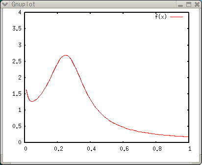
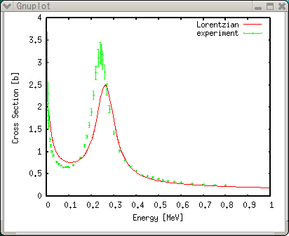
Introducing to gnuplot --- FunctionsUser-Defined FunctionsIf you can write an equation, gnuplot can calculate it. I mean, functions to be plotted are expressed in a simple functional form, for example, f(x)=a*x+b, and they do not contain a complicated integration / differentiation which needs a numerical calculation. Gnuplot has many basic functions such as sine, cosine, Bessel, Gamma, etc, and it can plot them as well as combinations of those functions. Maybe gnuplot users are not so interested in plotting functions, except for your Math homework (or some special purpose which I don't know), but this is extremely useful for a parameter-fitting to experimental data, namely a least-squares fitting. Gnuplot can solve not only linear least-squares problems but also non-linear ones. In this section, we learn how we can use a user-defined function, and how to fit this to experimental data. The function we are thinking here is the Lorentzian plus background term of 1/sqrt(x). This equation contains four parameters, a, b, c, and d, those are determined by experimental data.  Definition of a function is similar to Fortran or C programming language. In the example below, f(x)=c/((x-a)*(x-a)+b)+d/sqrt(x) defines our equation. Square of (x-a) term also can be written in a Fortran manner, (x-a)**2 . The parameters, a,b,c, and d are arbitrary. gnuplot> a=0.25 gnuplot> b=0.02 gnuplot> c=0.05 gnuplot> d=0.1 gnuplot> f(x)=c/((x-a)*(x-a)+b)+d/sqrt(x) gnuplot> set xrange [0:1] gnuplot> set yrange [0:4] gnuplot> plot f(x)  Values of the functionSince gnuplot calculates user-defined functions numerically to draw a graph on your screen, you can look at the calculated numbers with the print command. The value of function depends on the parameters (a,b,c,d, and e). Gnuplot calculates functions in a double-precision. gnuplot> print f(0.25) 2.7 gnuplot> print f(0.4) 1.33458447124371 gnuplot> a=0.4 gnuplot> print f(0.4) 2.65811388300842 To obtain the calculated values in a tabulated format, which can be processed with other applications such as a spread-sheet, use a special terminal table . To write the result, specify a file name with set output . gnuplot> set term table Terminal type set to 'table' gnuplot> plot f(x) #Curve 0, 100 points #x y type 0 0 u 0.010101 1.63972 i 0.020202 1.39031 i 0.030303 1.30688 i .... 0.979798 0.191506 i 0.989899 0.188622 i 1 0.185837 i gnuplot> set output "calc.plt" gnuplot> replot Search for the parameters with a Least-Squares MethodWe now fit the function to experimental data, and obtain best values of the parameters, a, b, c, and d. The experimental data are stored in a file "exp.dat". 2.5000E-03 3.0420E+00 6.47E-01 3.5000E-03 2.5700E+00 4.37E-01 4.5000E-03 2.3020E+00 2.53E-01 ... 7.0000E-01 2.7420E-01 2.14E-03 7.5000E-01 2.5680E-01 1.81E-03 8.0000E-01 2.4630E-01 1.59E-03 The data file consists of 3 columns, each of which is (x,y,z) data pair, the Z-data stand for an absolute uncertainty of the data Y. It means Z has the same dimension as Y. For example (in the case above), if your Y value is 3.04 cm, its uncertainty should be 0.647cm. The inverse of Z becomes a weight of this data point at the data fitting. If no uncertainty is given, the weights for all data points are the same. First of all, we show the data and function in one plot. As shown in Experimental Data or Numerical Calculation section, the axis names, ranges, tics, are adjusted properly. gnuplot> set xlabel "Energy [MeV]" gnuplot> set ylabel "Cross Section [b]" gnuplot> set xtics 0.1 gnuplot> set ytics 0.5 gnuplot> plot f(x) title "Lorentzian",\ > "exp.dat" using 1:2:3 title "experiment" with yerrors 
As I said that the parameters, a,b,c, and d, are arbitrary, but they were roughly determined for this experimental data. The parameter 'a' is a position of Lorentzian peak, and which is, say, about 0.25 from this plotting. For the parameter 'b', its square-root corresponds to the width of this peak, and I estimated that b is about 0.02. It is quite easy to do a least-squares fitting with gnuplot. Just use the fit command, and add parameters to be searched for by the via option. When your fitting function is strongly non-linear, you need to be careful about the initial values of your parameters. Here we used the values above as the initial parameters for this fitting.
gnuplot> fit f(x) "exp.dat" using 1:2:3 via a,b,c,d


Iteration 0
WSSR        : 96618.1           delta(WSSR)/WSSR   : 0
delta(WSSR) : 0                 limit for stopping : 1e-05
lambda    : 1150.73

initial set of free parameter values

    ...

After 17 iterations the fit converged.
final sum of squares of residuals : 3341.93
rel. change during last iteration : -5.29173e-06

degrees of freedom (ndf) : 47
rms of residuals      (stdfit) = sqrt(WSSR/ndf)      : 8.43237
variance of residuals (reduced chisquare) = WSSR/ndf : 71.1049

Final set of parameters            Asymptotic Standard Error
=======================            ==========================

a               = 0.26191          +/- 0.005759     (2.199%)
b               = 0.00251445       +/- 0.0008358    (33.24%)
c               = 0.00541346       +/- 0.0009206    (17.01%)
d               = 0.182469         +/- 0.007329     (4.016%)


correlation matrix of the fit parameters:

               a      b      c      d
a               1.000
b               0.042  1.000
c              -0.229  0.783  1.000
d               0.210 -0.538 -0.768  1.000
gnuplot> replot
 As shown above, the fitted function is not so good except for the region where the data are off-resonance. This is because our fitting function was not the best choice. Its peak shape looks fine with the Lorentzian, so we modify d/sqrt(x) by introducing a new parameter 'e' and express it as d*x**e . The initial value of 'e' is -0.5.
gnuplot> e=-0.5
gnuplot> f(x)=c/((x-a)*(x-a)+b)+d*x**e
gnuplot> fit f(x) "exp.dat" using 1:2:3 via a,b,c,d,e

     ...
Final set of parameters            Asymptotic Standard Error
=======================            ==========================

a               = 0.25029          +/- 0.002106     (0.8412%)
b               = 0.00197707       +/- 0.0002747    (13.89%)
c               = 0.00550098       +/- 0.0003662    (6.657%)
d               = 0.21537          +/- 0.003743     (1.738%)
e               = -0.358371        +/- 0.0115       (3.208%)


correlation matrix of the fit parameters:

               a      b      c      d      e
a               1.000
b               0.021  1.000
c              -0.078  0.788  1.000
d              -0.110 -0.384 -0.500  1.000
e              -0.304  0.198  0.335  0.381  1.000
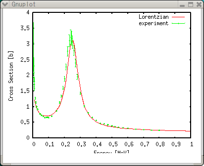
gnuplot> replot

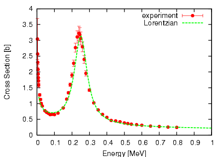
Still its not perfect. Fixing a=0.24 and search only for via b,c,d,e gives you better looks, but its chi-square is larger. Output in the Postscript formatAs shown in Experimental Data section. we generate a Postscript figure. The data points are drawn with solid line and seventh symbol (circle), and the function is shown with the thick dashed line. gnuplot> set linestyle 1 lt 1 pt 7 gnuplot> set linestyle 2 lt 2 lw 3 gnuplot> set size 0.6,0.6 gnuplot> set term postscript eps enhanced color Terminal type set to 'postscript' Options are 'eps enhanced color dashed defaultplex "Helvetica" 14' gnuplot> set output "exp.ps" gnuplot> plot"exp.dat" using 1:2:3 title "experiment" with yerrors ls 1,\ > f(x) title "Lorentzian" with line ls 2  |